只需一步,轻松用Python实现线性规划
线性规划说明
什么是线性规划?
什么是混合整数线性规划?
为什么线性规划很重要?
Gurobi 优化案例研究 线性规划技术的五个应用领域
使用 Python 进行线性规划
构建 Python C 扩展模块 CPython 内部 用 C 或 C++ 扩展 Python
SciPy Optimization and Root Finding PuLP Pyomo CVXOPT
线性规划示例
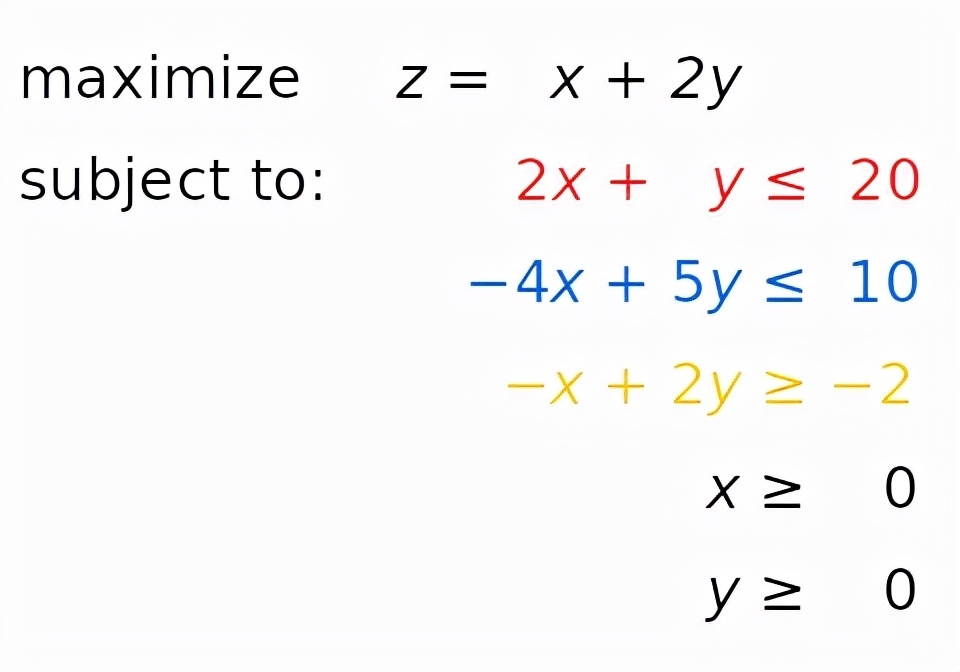
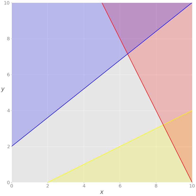
小型线性规划问题
不可行的线性规划问题
无界线性规划问题
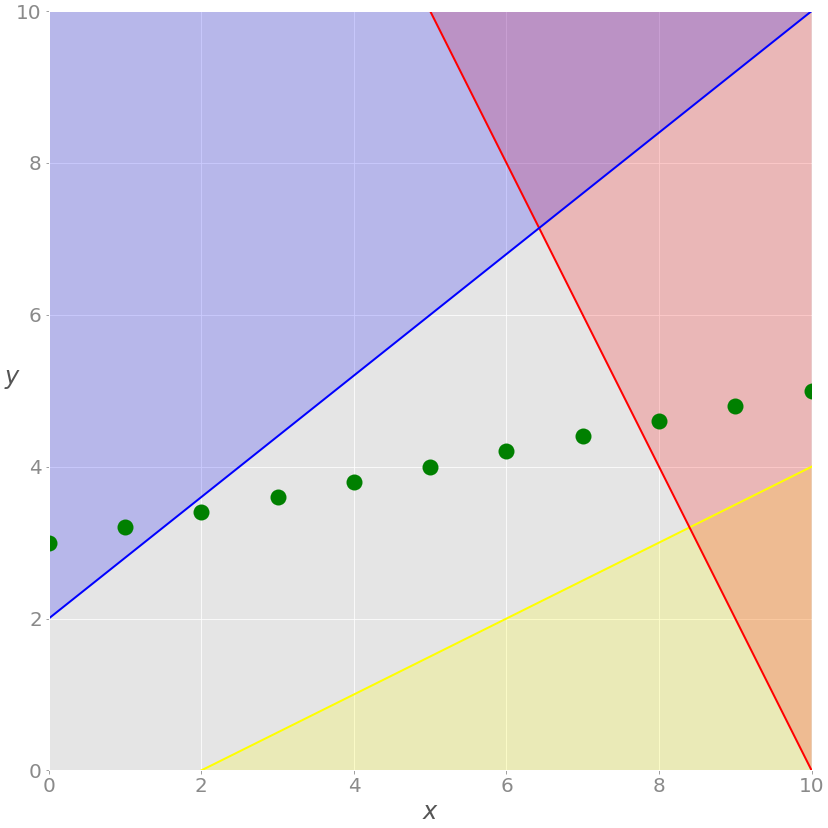
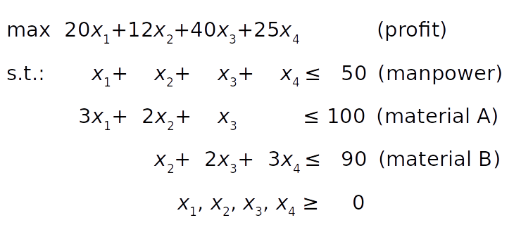
资源分配问题
线性规划 Python 实现
安装 SciPy 和 PuLP
$ python -m pip install -U "scipy==1.4.*" "pulp==2.1"$ pulptest$ brew install glpk$ sudo apt install glpk glpk-utils$ sudo dnf install glpk-utils$ conda install -c conda-forge glpk$ glpsol --version使用 SciPy
>>>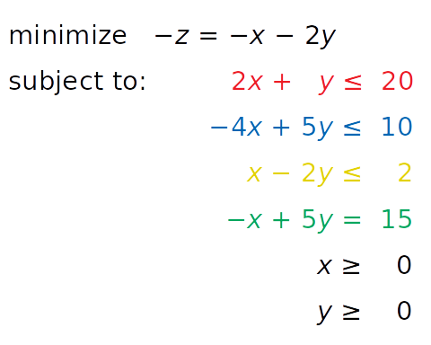
>>> from scipy.optimize import linprog示例 1
不是最大化z = x + 2 y,你可以最小化它的负值(− z = − x − 2 y)。 代替大于或等于符号,您可以将黄色不等式乘以 -1 并得到小于或等于符号 (≤) 的相反数。
>>>
>>> obj = [-1, -2]
>>> # ─┬ ─┬
>>> # │ └┤ Coefficient for y
>>> # └────┤ Coefficient for x
>>> lhs_ineq = [[ 2, 1], # Red constraint left side
... [-4, 5], # Blue constraint left side
... [ 1, -2]] # Yellow constraint left side
>>> rhs_ineq = [20, # Red constraint right side
... 10, # Blue constraint right side
... 2] # Yellow constraint right side
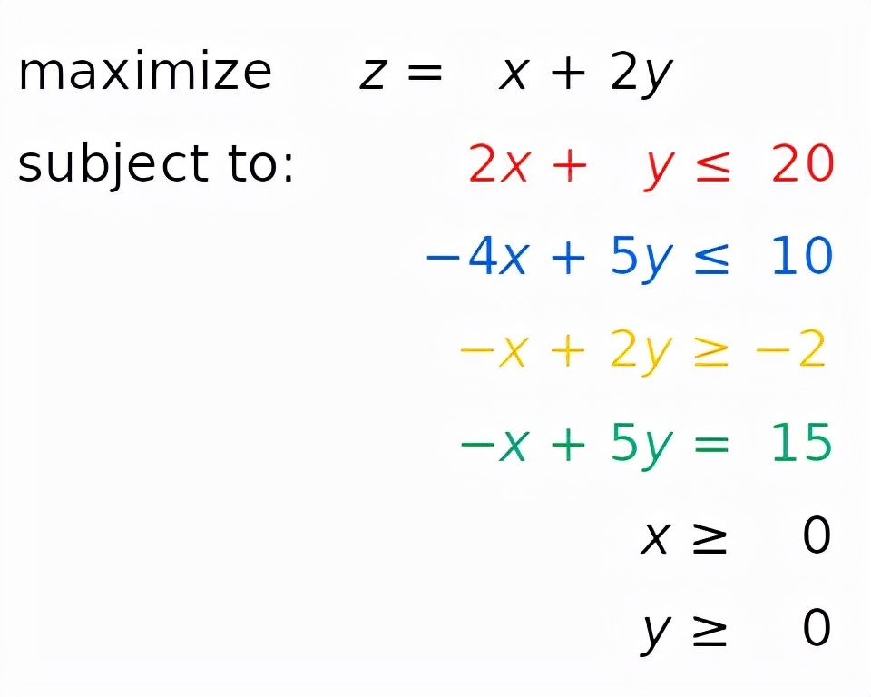
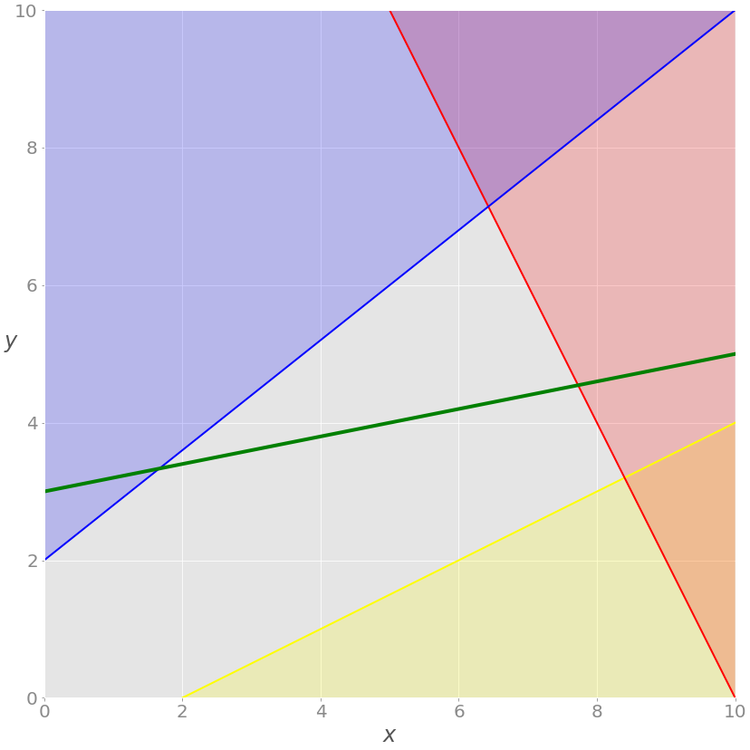
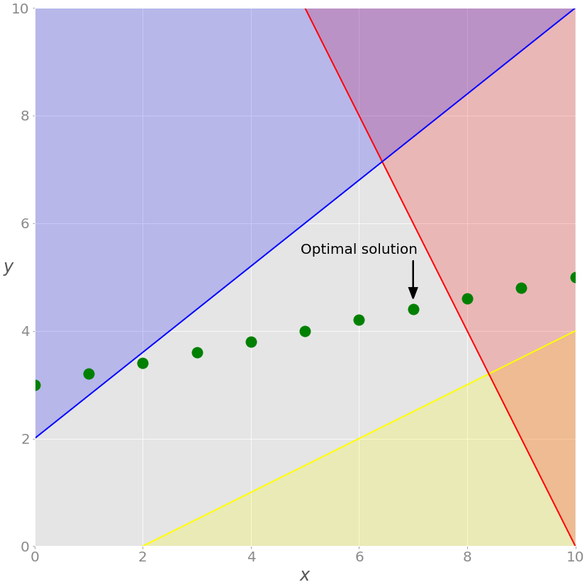
>>> lhs_eq = [[-1, 5]] # Green constraint left side
>>> rhs_eq = [15] # Green constraint right sideobj 保存目标函数的系数。 lhs_ineq 保存不等式(红色、蓝色和黄色)约束的左侧系数。 rhs_ineq 保存不等式(红色、蓝色和黄色)约束的右侧系数。 lhs_eq 保存来自等式(绿色)约束的左侧系数。 rhs_eq 保存来自等式(绿色)约束的右侧系数。
>>>
>>> bnd = [(0, float("inf")),  # Bounds of x
... (0, float("inf"))] # Bounds of y>>>
>>> opt = linprog(c=obj, A_ub=lhs_ineq, b_ub=rhs_ineq,
... A_eq=lhs_eq, b_eq=rhs_eq, bounds=bnd,
... method="revised simplex")
>>> opt
con: array([0.])
fun: -16.818181818181817
message: 'Optimization terminated successfully.'
nit: 3
slack: array([ 0. , 18.18181818, 3.36363636])
status: 0
success: True
x: array([7.72727273, 4.54545455]).con 是等式约束残差。 .fun 是最优的目标函数值(如果找到)。 .message 是解决方案的状态。 .nit 是完成计算所需的迭代次数。 .slack 是松弛变量的值,或约束左右两侧的值之间的差异。 .status 是一个介于0和之间的整数4,表示解决方案的状态,例如0找到最佳解决方案的时间。 .success 是一个布尔值,显示是否已找到最佳解决方案。 .x 是一个保存决策变量最优值的 NumPy 数组。
>>>
>>> opt.fun
-16.818181818181817

>>> opt.success
True

>>> opt.x
array([7.72727273, 4.54545455])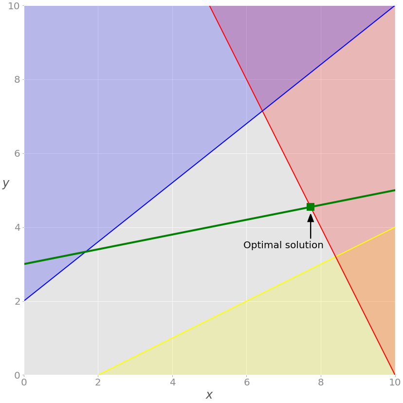
>>>
>>> opt = linprog(c=obj, A_ub=lhs_ineq, b_ub=rhs_ineq, bounds=bnd,
...               method="revised simplex")
>>> opt
     con: array([], dtype=float64)
     fun: -20.714285714285715
 message: 'Optimization terminated successfully.'
     nit: 2
   slack: array([0.        , 0.        , 9.85714286])
  status: 0
 success: True
       x: array([6.42857143, 7.14285714]))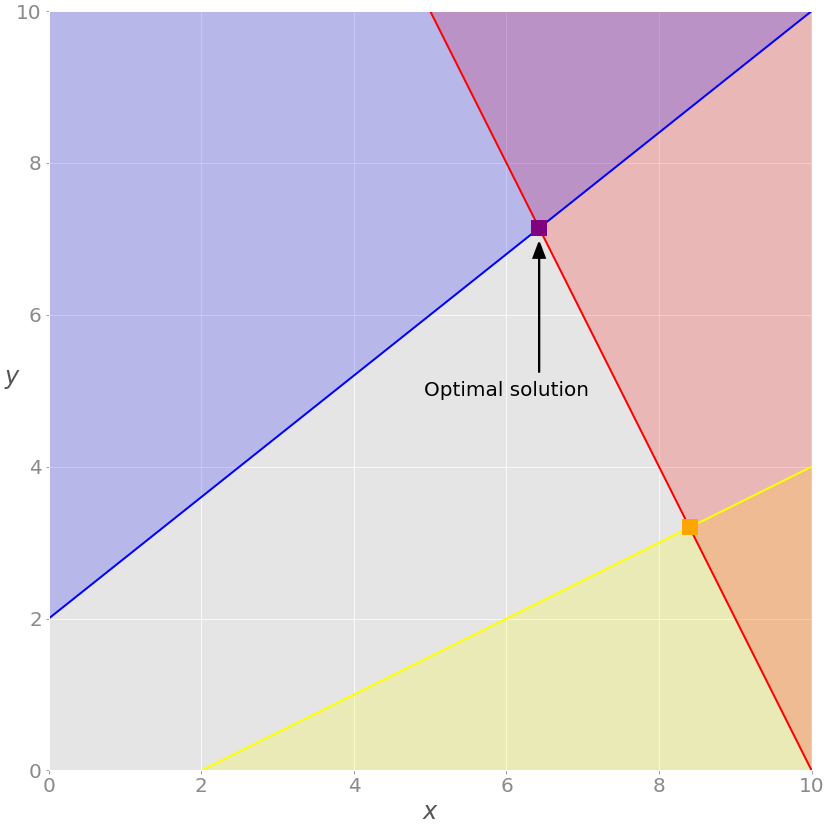
示例 2
>>>
>>> obj = [-20, -12, -40, -25]

>>> lhs_ineq = [[1, 1, 1, 1],  # Manpower
...             [3, 2, 1, 0],  # Material A
...             [0, 1, 2, 3]]  # Material B

>>> rhs_ineq = [ 50,  # Manpower
...             100,  # Material A
...              90]  # Material B

>>> opt = linprog(c=obj, A_ub=lhs_ineq, b_ub=rhs_ineq,
...               method="revised simplex")
>>> opt
     con: array([], dtype=float64)
     fun: -1900.0
 message: 'Optimization terminated successfully.'
     nit: 2
   slack: array([ 0., 40.,  0.])
  status: 0
 success: True
x: array([ 5., 0., 45., 0.])SciPy 无法运行各种外部求解器。 SciPy 不能使用整数决策变量。 SciPy 不提供促进模型构建的类或函数。您必须定义数组和矩阵,这对于大型问题来说可能是一项乏味且容易出错的任务。 SciPy 不允许您直接定义最大化问题。您必须将它们转换为最小化问题。 SciPy 不允许您直接使用大于或等于符号来定义约束。您必须改用小于或等于。
Using PuLP
from pulp import LpMaximize, LpProblem, LpStatus, lpSum, LpVariable示例 1
# Create the model
model = LpProblem(name="small-problem", sense=LpMaximize)# Initialize the decision variables
x = LpVariable(name="x", lowBound=0)
y = LpVariable(name="y", lowBound=0)>>>
>>> expression = 2 * x + 4 * y
>>> type(expression)
>>> constraint = 2 * x + 4 * y >= 8
>>> type(constraint)
# Add the constraints to the model
model += (2 * x + y <= 20, "red_constraint")
model += (4 * x - 5 * y >= -10, "blue_constraint")
model += (-x + 2 * y >= -2, "yellow_constraint")
model += (-x + 5 * y == 15, "green_constraint")# Add the objective function to the model
obj_func = x + 2 * y
model += obj_func# Add the objective function to the model
model += x + 2 * y# Add the objective function to the model
model += lpSum([x, 2 * y])>>>
>>> model
small-problem:
MAXIMIZE
1*x + 2*y + 0
SUBJECT TO
red_constraint: 2 x + y <= 20
blue_constraint: 4 x - 5 y >= -10
yellow_constraint: - x + 2 y >= -2
green_constraint: - x + 5 y = 15
VARIABLES
x Continuous
y Continuous# Solve the problem
status = model.solve()>>>
>>> print(f"status: {model.status}, {LpStatus[model.status]}")
status: 1, Optimal
>>> print(f"objective: {model.objective.value()}")
objective: 16.8181817
>>> for var in model.variables():
... print(f"{var.name}: {var.value()}")
...
x: 7.7272727
y: 4.5454545
>>> for name, constraint in model.constraints.items():
... print(f"{name}: {constraint.value()}")
...
red_constraint: -9.99999993922529e-08
blue_constraint: 18.181818300000003
yellow_constraint: 3.3636362999999996
green_constraint: -2.0000000233721948e-07)>>>
>>> model.variables()
[x, y]
>>> model.variables()[0] is x
True
>>> model.variables()[1] is y
True>>>
>>> model.solver
from pulp import GLPK# Create the model
model = LpProblem(name="small-problem", sense=LpMaximize)
# Initialize the decision variables
x = LpVariable(name="x", lowBound=0)
y = LpVariable(name="y", lowBound=0)
# Add the constraints to the model
model += (2 * x + y <= 20, "red_constraint")
model += (4 * x - 5 * y >= -10, "blue_constraint")
model += (-x + 2 * y >= -2, "yellow_constraint")
model += (-x + 5 * y == 15, "green_constraint")
# Add the objective function to the model
model += lpSum([x, 2 * y])
# Solve the problem
status = model.solve(solver=GLPK(msg=False))>>>
>>> print(f"status: {model.status}, {LpStatus[model.status]}")
status: 1, Optimal
>>> print(f"objective: {model.objective.value()}")
objective: 16.81817
>>> for var in model.variables():
... print(f"{var.name}: {var.value()}")
...
x: 7.72727
y: 4.54545
>>> for name, constraint in model.constraints.items():
... print(f"{name}: {constraint.value()}")
...
red_constraint: -1.0000000000509601e-05
blue_constraint: 18.181830000000005
yellow_constraint: 3.3636299999999997
green_constraint: -2.000000000279556e-05>>>
>>> model.solver
# Create the model
model = LpProblem(name="small-problem", sense=LpMaximize)
# Initialize the decision variables: x is integer, y is continuous
x = LpVariable(name="x", lowBound=0, cat="Integer")
y = LpVariable(name="y", lowBound=0)
# Add the constraints to the model
model += (2 * x + y <= 20, "red_constraint")
model += (4 * x - 5 * y >= -10, "blue_constraint")
model += (-x + 2 * y >= -2, "yellow_constraint")
model += (-x + 5 * y == 15, "green_constraint")
# Add the objective function to the model
model += lpSum([x, 2 * y])
# Solve the problem
status = model.solve()>>>
>>> print(f"status: {model.status}, {LpStatus[model.status]}")
status: 1, Optimal
>>> print(f"objective: {model.objective.value()}")
objective: 15.8
>>> for var in model.variables():
... print(f"{var.name}: {var.value()}")
...
x: 7.0
y: 4.4
>>> for name, constraint in model.constraints.items():
... print(f"{name}: {constraint.value()}")
...
red_constraint: -1.5999999999999996
blue_constraint: 16.0
yellow_constraint: 3.8000000000000007
green_constraint: 0.0)
>>> model.solver
示例 2
# Define the model
model = LpProblem(name="resource-allocation", sense=LpMaximize)

# Define the decision variables
x = {i: LpVariable(name=f"x{i}", lowBound=0) for i in range(1, 5)}

# Add constraints
model += (lpSum(x.values()) <= 50, "manpower")
model += (3 * x[1] + 2 * x[2] + x[3] <= 100, "material_a")
model += (x[2] + 2 * x[3] + 3 * x[4] <= 90, "material_b")

# Set the objective
model += 20 * x[1] + 12 * x[2] + 40 * x[3] + 25 * x[4]

# Solve the optimization problem
status = model.solve()

# Get the results
print(f"status: {model.status}, {LpStatus[model.status]}")
print(f"objective: {model.objective.value()}")

for var in x.values():
    print(f"{var.name}: {var.value()}")

for name, constraint in model.constraints.items():
print(f"{name}: {constraint.value()}")status: 1, Optimal
objective: 1900.0
x1: 5.0
x2: 0.0
x3: 45.0
x4: 0.0
manpower: 0.0
material_a: -40.0
material_b: 0.0 1model = LpProblem(name="resource-allocation", sense=LpMaximize)
2
3# Define the decision variables
4x = {i: LpVariable(name=f"x{i}", lowBound=0) for i in range(1, 5)}
5y = {i: LpVariable(name=f"y{i}", cat="Binary") for i in (1, 3)}
6
7# Add constraints
8model += (lpSum(x.values()) <= 50, "manpower")
9model += (3 * x[1] + 2 * x[2] + x[3] <= 100, "material_a")
10model += (x[2] + 2 * x[3] + 3 * x[4] <= 90, "material_b")
11
12M = 100
13model += (x[1] <= y[1] * M, "x1_constraint")
14model += (x[3] <= y[3] * M, "x3_constraint")
15model += (y[1] + y[3] <= 1, "y_constraint")
16
17# Set objective
18model += 20 * x[1] + 12 * x[2] + 40 * x[3] + 25 * x[4]
19
20# Solve the optimization problem
21status = model.solve()
22
23print(f"status: {model.status}, {LpStatus[model.status]}")
24print(f"objective: {model.objective.value()}")
25
26for var in model.variables():
27 print(f"{var.name}: {var.value()}")
28
29for name, constraint in model.constraints.items():
30 print(f"{name}: {constraint.value()}")第 5 行 定义了二元决策变量y[1]并y[3]保存在字典中y。 第 12 行 定义了一个任意大的数M。100在这种情况下,该值足够大,因为您100每天的数量不能超过单位。 第 13 行 说如果y[1]为零,则x[1]必须为零,否则它可以是任何非负数。 第 14 行 说如果y[3]为零,则x[3]必须为零,否则它可以是任何非负数。 第 15 行 说要么y[1]ory[3]为零(或两者都是),所以要么x[1]or 也x[3]必须为零。
status: 1, Optimal
objective: 1800.0
x1: 0.0
x2: 0.0
x3: 45.0
x4: 0.0
y1: 0.0
y3: 1.0
manpower: -5.0
material_a: -55.0
material_b: 0.0
x1_constraint: 0.0
x3_constraint: -55.0
y_constraint: 0.0线性规划求解器
GLPK LP Solve CLP CBC CVXOPT SciPy SCIP with PySCIPOpt Gurobi Optimizer CPLEX XPRESS MOSEK
结论
原文链接:https://bbs.huaweicloud.com/blogs/317032?utm_source=cnblog&utm_medium=bbs-ex&utm_campaign=other&utm_content=content
作者:Yuchuan